
3dv入门—3D Gaussian Splatting
Published:
听群友这样说,在3dv 2024会议上,3DGS一作讲论文的时候NeRF一作进来发现没位置了,还被关门外了
3D Gaussian Splatting
整体的框架
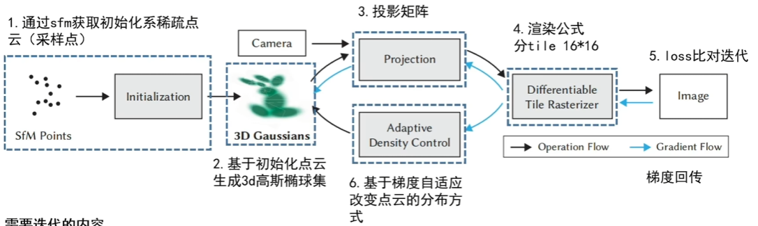
SFM,structure from motion,中文直译名就是运动恢复结构,可以重建稀疏点云的和相机参数(内外),其应用最多的场景还是用于标定相机的内外参数,这也是为什么我们可以直接从视频中进行抽帧的原因。
初始稀疏点云
与NeRF中相同,我们首先要使用colmap进行创建一个稀疏的初始化的点云,如下图所示,通过一组图片去计算每一组图片的位姿,从而最后得到一些稀疏的关键点云;
有意思的是,这里生成的点云只是3DGS中场景中初始化默认的一些点,由于后续还会有梯度回传到点云里,因此这里点云甚至可以随机初始化出来,就是可能导致收敛时间更长了些。

3D高斯椭球集的创建—-位置与形状
位置信息:点云位置信息优化,也就是$(x,y,z)$,即高斯椭球的中心点均值$\mu$
形状信息:高斯椭球的协方差矩阵$\Sigma$,$\Sigma$包含高斯椭球的旋转矩阵$R$和在各个轴的缩放矩阵$S$,其中$\Sigma = RSS^TR^T$。
3D高斯椭球集的创建—-颜色与不透明度
颜色信息:点云颜色$(r,g,b)$—-使用球谐函数来表示,使得点云在不同的角度会呈现不同的颜色,而且有利于提高迭代的效率(在代码中使用4阶来表示)
不透明度信息:点云的不透明度,密度优化$\alpha$
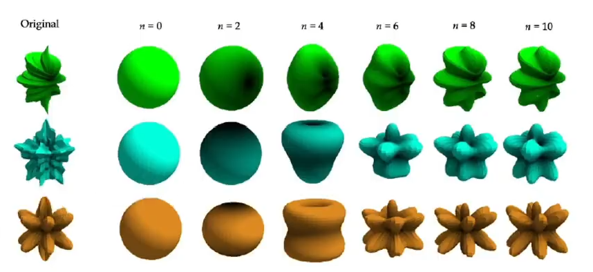
关于球谐函数
球谐函数可以看作是一种多项式的拟合(泰勒展开式),在多项式的拟合中,表达能力会随着阶数的能力的提升而提高;例如$f(x) = ax^3+bx^2+cx^1+dx^0$中,$x^3,x^2,x^1,x^0$分别代表基函数。
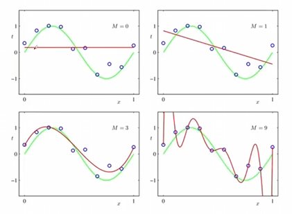
而傅里叶级数的展开,其实就是使用了$sinx$和$cosx$这样的基函数去拟合出不同的周期函数。而球谐函数,就是一个用在球面上的基函数,用于去拟合球面上不停变换的离散的值,其阶数越高,表达能力会越强。
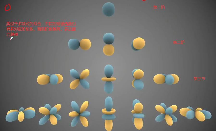
球谐函数是什么我们先不用管,先了解球谐函数只与$\theta$和$\phi$有关,
“这玩意直接拟合三维点云不就有密集三维模型了吗”
对这些球谐函数的基函数进行加权组合,得到球面上的一组函数,从而有效地将离散的数据转化为连续的数据。
在3DGS中,点云颜色$(r,g,b)$是使用球谐函数来表示的,使得点云在不同的角度可以呈现不同的颜色,并且这样有利于提高迭代的效率。
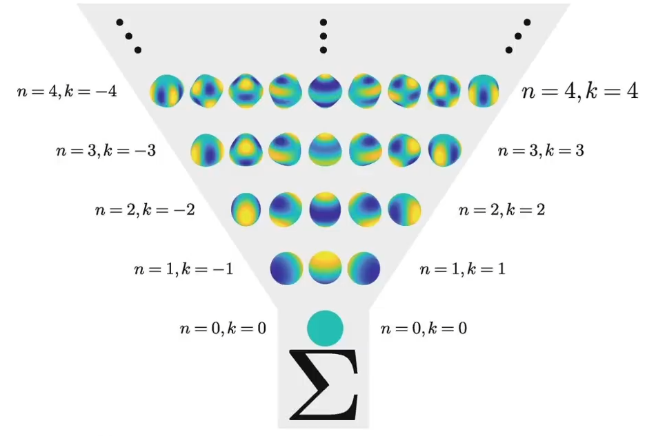
在3DGS的实际过程中,点云颜色使用了4阶的球谐函数进行表示,$n$阶球谐函数的参数量为$n^2$,如果是R,G,B三个值,那么就是3*16,一共有48个属性,组合之后,可以将离散的颜色数据转化为连续的颜色数据,同时有利于对参数进行迭代
3D高斯椭球集的创建
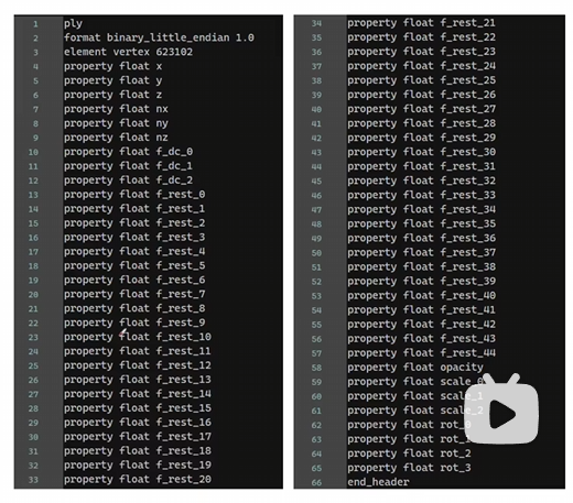
其中element vertex是跑出来多少点数,然后每个点拥有下面这六十行的属性,其中(x,y,z)是位置信息,也就是中心点\mu,(nx,ny,nz)是指法向量信息,但是好像没有用到?从f_dc_0到f_dc_2是代表每个高斯分布的颜色RGB的球谐系数(SH)以及(f_rest_0 到 f_rest_44),一共是3+45个属性,平均到每个RGB就是16个属性。opacity就是不透明度信息$\alpha$,scale_0,scale_1,scale_2就是三个方向的缩放矩阵,也即协方差矩阵的参数,从rot_0到rot_3是旋转矩阵,使用旋转四元数(一个实部和三个虚部来组成的)来进行表示。
计算机图形学投影矩阵
渲染公式
首先回顾NeRF的体渲染公式,连续的是这个样子,在这一篇blog我们相对详细地讨论了这个:
\[C=\sum_{i=1}^NT_i(1-\exp(-\sigma_i\delta_i))\mathbf{c}_i\quad\mathrm{with}\quad T_i=\exp\left(-\sum_{j=1}^{i-1}\sigma_j\delta_j\right)\]离散化之后是这样的:
\[C=\sum_{i=1}^NT_i\alpha_i\mathbf{c}_i,\quad\text{with}\quad\alpha_i=(1-\exp(-\sigma_i\delta_i)) \text{and} T_i=\prod_{j=1}^{i-1}(1-\alpha_i)\]在NeRF中,是通过对生成的射线上进行点的采样得到,但是在3DGS中,也是基于类似的这样基于”点”的方法,也即通过点云中一定的半径范围中能影响像素的N个有序的点来计算一个像素的颜色$c$:
\[C=\sum_{i\in N}c_{i}\alpha_{i}\prod_{j=1}^{i-1}(1-\alpha_{j})\]其中,$a_{i}$代表当前点i的不透明度(密度)值,$a_{j}$代表$i$之前的点的不透明度值,使用$1-a_{j}$的累乘,作为权重weight,这实际是代表前面的点越透明,这个weight会越大,当前a_{i}的影响权重就会越大。
损失Loss定义
与NeRF相同,其损失函数定义同样十分简单:
\[\mathcal{L}=(1-\lambda)\mathcal{L}_1+\lambda\mathcal{L}_\text{D-SSIM}\]其中L1损失与NeRF中的类似,用于评价重建前后的损失情况,D-SSIM是一个类似的评价图像质量损失的loss函数。
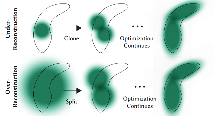
基于梯度自适应改变点云的分布方式
每隔100个epoch会去判断点云的分布是否是合理的。
- Pruning掉一些透明度很高的点,或者离相机比较近的一些点
- 过度重构和欠采样(基于梯度来进行判断)
- 如果是过度重构,方差(?)很小,通过克隆高斯来适应 ( Under-Reconstruction
- 如果是欠采样,方差很大,就通过分割高斯来进行适应 ( Over-Reconstruction
3DGS代码解析
Rander函数的过程
def render(viewpoint_camera, pc : GaussianModel, pipe, bg_color : torch.Tensor, scaling_modifier = 1.0, override_color = None):
    """
    Render the scene.

    Background tensor (bg_color) must be on GPU!

    这里的pipe是什么意思
    """
    # Create zero tensor. We will use it to make pytorch return gradients of the 2D (screen-space) means
    # 创建一个与输入点云(高斯模型)大小相同的零张量,用于记录屏幕空间中的点的位置。这个张量将用于计算对于屏幕空间坐标的梯度。
    screenspace_points = torch.zeros_like(pc.get_xyz, dtype=pc.get_xyz.dtype, requires_grad=True, device="cuda") + 0
    try:
        screenspace_points.retain_grad()  #  #尝试保留张量的梯度。这是为了确保可以在反向传播过程中计算对于屏幕空间坐标的梯度。
    except:
        pass

    # Set up rasterization configuration
    # 计算视场的 tan 值,这将用于设置光栅化配置。   话说这里为什么要计算tan
    tanfovx = math.tan(viewpoint_camera.FoVx * 0.5)
    tanfovy = math.tan(viewpoint_camera.FoVy * 0.5)

    # 设置光栅化的配置,包括图像的大小、视场的 tan 值、背景颜色、视图矩阵、投影矩阵等。
    raster_settings = GaussianRasterizationSettings(
        image_height=int(viewpoint_camera.image_height),
        image_width=int(viewpoint_camera.image_width),
        tanfovx=tanfovx,
        tanfovy=tanfovy,
        bg=bg_color,
        scale_modifier=scaling_modifier,
        viewmatrix=viewpoint_camera.world_view_transform,
        projmatrix=viewpoint_camera.full_proj_transform,
        sh_degree=pc.active_sh_degree,   # 这里的sh代表球谐函数
        campos=viewpoint_camera.camera_center,
        prefiltered=False,
        debug=pipe.debug
    )

    # 创建一个高斯光栅化器对象,用于将高斯分布投影到屏幕上。    好像可以和ai葵说的那些联系起来
    rasterizer = GaussianRasterizer(raster_settings=raster_settings)

    # 获取高斯分布的三维坐标、屏幕空间坐标和透明度。
    means3D = pc.get_xyz
    means2D = screenspace_points
    opacity = pc.get_opacity

    # 如果提供了预先计算的3D协方差矩阵,则使用它。否则,它将由光栅化器根据尺度和旋转进行计算。
    scales = None
    rotations = None
    cov3D_precomp = None
    if pipe.compute_cov3D_python:   # 如果提供了就直接获取
        cov3D_precomp = pc.get_covariance(scaling_modifier)
    else:                           # 如果没有直接提供,就通过一个仿射变换去获取?
        scales = pc.get_scaling
        rotations = pc.get_rotation

    # 如果提供了预先计算的颜色,则使用它们。否则,如果希望在Python中从球谐函数中预计算颜色,请执行此操作。
    # 如果没有,则颜色将通过光栅化器进行从球谐函数到RGB的转换。
    shs = None
    colors_precomp = None
    if override_color is None:
        if pipe.convert_SHs_python:   # SH是什么,是球谐函数
            shs_view = pc.get_features.transpose(1, 2).view(-1, 3, (pc.max_sh_degree+1)**2)  # 将SH特征的形状调整为(batch_size * num_points,3,(max_sh_degree+1)**2)。
            dir_pp = (pc.get_xyz - viewpoint_camera.camera_center.repeat(pc.get_features.shape[0], 1))
            dir_pp_normalized = dir_pp/dir_pp.norm(dim=1, keepdim=True)
            sh2rgb = eval_sh(pc.active_sh_degree, shs_view, dir_pp_normalized)
            colors_precomp = torch.clamp_min(sh2rgb + 0.5, 0.0)
        else:
            shs = pc.get_features
    else:
        colors_precomp = override_color

    # Rasterize visible Gaussians to image, obtain their radii (on screen).
    # 调用光栅化器,将高斯分布投影到屏幕上,获得渲染图像和每个高斯分布在屏幕上的半径。  这个操作似乎是在diff_gaussian_rasterization这个库中实现的,这个库有空去看看ai葵的讲解
    rendered_image, radii = rasterizer(
        means3D = means3D,
        means2D = means2D,
        shs = shs,
        colors_precomp = colors_precomp,
        opacities = opacity,
        scales = scales,
        rotations = rotations,
        cov3D_precomp = cov3D_precomp)

    # Those Gaussians that were frustum culled or had a radius of 0 were not visible.
    # They will be excluded from value updates used in the splitting criteria.
    # 返回一个字典,包含渲染的图像、屏幕空间坐标、可见性过滤器(根据半径判断是否可见)以及每个高斯分布在屏幕上的半径。
    return {"render": rendered_image,
            "viewspace_points": screenspace_points,
            "visibility_filter" : radii > 0,
            "radii": radii}
在这段代码中,描述了生成的高斯点投影到2D屏幕上的过程,这里最为核心的地自然是其创建的GaussianRasterizer高斯光栅化器对象,然而想要搞明白具体的投影过程的实现,还是要深入cuda代码去看一下,整个过程可以被简单的描述为计算投影后的半径->计算出来⚪覆盖了哪些像素->搞明白高斯的顺序->计算每个像素的颜色。
打开cuda_resterizer这个文件,我们很容易注意到有backward.cu和forward.cu这两个文件,这也是与torch框架的最大不同处,也就是反向传播还要自己算出来再写上,
- 计算投影后⚪近似的半径
这部分的重点在与怎么把一个个3d的椭球投影到平面上(其实这里为了方便是简化(近似)保存的一个一个的⚪,因为⚪只需要记录好其中心和半径即可了。
针对于每个像素,投影到高斯上的像素的数量是不一样的,因此无法使用pytorch来很好的将这个东西进行平行化。使用pytorch进行计算的前提是要保持每个像素的计算都是相同的,这也是为什么作者使用了CUDA。
- 计算出来⚪覆盖了哪些像素 在投影的过程中,整个图片会被切分为很多个小格子,然后会计算投影的⚪跟哪些小格子是有交汇的,然后会把这个小格子里所有的像素都认定为与这个像素是有交集的,这样其实是使得被列入计算,被认为有交集的像素多了很多。
这两个步骤主要是由在forward.cu代码文件中的processCUDA函数实现的:
// Perform initial steps for each Gaussian prior to rasterization.
template<int C>
__global__ void preprocessCUDA(int P, int D, int M,
	const float* orig_points,
	const glm::vec3* scales,
	const float scale_modifier,
	const glm::vec4* rotations,
	const float* opacities,
	const float* shs,
	bool* clamped,
	const float* cov3D_precomp,
	const float* colors_precomp,
	const float* viewmatrix,
	const float* projmatrix,
	const glm::vec3* cam_pos,
	const int W, int H,
	const float tan_fovx, float tan_fovy,
	const float focal_x, float focal_y,
	int* radii,
	float2* points_xy_image,
	float* depths,
	float* cov3Ds,
	float* rgb,
	float4* conic_opacity,
	const dim3 grid,
	uint32_t* tiles_touched,
	bool prefiltered)
{
	auto idx = cg::this_grid().thread_rank();
	if (idx >= P)
		return;

	// Initialize radius and touched tiles to 0. If this isn't changed,
	// this Gaussian will not be processed further.
	radii[idx] = 0;
	tiles_touched[idx] = 0;

	// Perform near culling, quit if outside.
	float3 p_view;
	if (!in_frustum(idx, orig_points, viewmatrix, projmatrix, prefiltered, p_view))
		return;

	// Transform point by projecting

  // 把3D点投影到矩阵上
	float3 p_orig = { orig_points[3 * idx], orig_points[3 * idx + 1], orig_points[3 * idx + 2] };
	float4 p_hom = transformPoint4x4(p_orig, projmatrix);
	float p_w = 1.0f / (p_hom.w + 0.0000001f);
	float3 p_proj = { p_hom.x * p_w, p_hom.y * p_w, p_hom.z * p_w };

	// If 3D covariance matrix is precomputed, use it, otherwise compute
	// from scaling and rotation parameters.
	const float* cov3D;
	if (cov3D_precomp != nullptr)
	{
		cov3D = cov3D_precomp + idx * 6;   // 计算三个轴的长度是多少的过程.
	}
	else
	{
		computeCov3D(scales[idx], scale_modifier, rotations[idx], cov3Ds + idx * 6);
		cov3D = cov3Ds + idx * 6;
	}

  // 计算椭球投影到2D后 的长度是多少的过程
	// Compute 2D screen-space covariance matrix    计算投影的过程
	float3 cov = computeCov2D(p_orig, focal_x, focal_y, tan_fovx, tan_fovy, cov3D, viewmatrix);

	// Invert covariance (EWA algorithm)
	float det = (cov.x * cov.z - cov.y * cov.y);
	if (det == 0.0f)
		return;
	float det_inv = 1.f / det;
	float3 conic = { cov.z * det_inv, -cov.y * det_inv, cov.x * det_inv };

	// Compute extent in screen space (by finding eigenvalues of
	// 2D covariance matrix). Use extent to compute a bounding rectangle
	// of screen-space tiles that this Gaussian overlaps with. Quit if
	// rectangle covers 0 tiles.
	float mid = 0.5f * (cov.x + cov.z);
	float lambda1 = mid + sqrt(max(0.1f, mid * mid - det));   // 长轴半径
	float lambda2 = mid - sqrt(max(0.1f, mid * mid - det));   // 短轴半径
	float my_radius = ceil(3.f * sqrt(max(lambda1, lambda2)));   //
	float2 point_image = { ndc2Pix(p_proj.x, W), ndc2Pix(p_proj.y, H) };
	uint2 rect_min, rect_max;
	getRect(point_image, my_radius, rect_min, rect_max, grid);    // 计算每个圆覆盖了哪些像素
	if ((rect_max.x - rect_min.x) * (rect_max.y - rect_min.y) == 0)
		return;

	// If colors have been precomputed, use them, otherwise convert
	// spherical harmonics coefficients to RGB color.
	if (colors_precomp == nullptr)
	{
		glm::vec3 result = computeColorFromSH(idx, D, M, (glm::vec3*)orig_points, *cam_pos, shs, clamped);
		rgb[idx * C + 0] = result.x;
		rgb[idx * C + 1] = result.y;
		rgb[idx * C + 2] = result.z;
	}

	// Store some useful helper data for the next steps.
	depths[idx] = p_view.z;
	radii[idx] = my_radius;
	points_xy_image[idx] = point_image;
	// Inverse 2D covariance and opacity neatly pack into one float4
	conic_opacity[idx] = { conic.x, conic.y, conic.z, opacities[idx] };
	tiles_touched[idx] = (rect_max.y - rect_min.y) * (rect_max.x - rect_min.x);
}
- 计算每个高斯的前后顺序
…
- 计算每个像素的颜色
…
- 实现高斯的删除和新增
    def prune_points(self, mask): # 删除Gaussian并移除对应的所有属性
        valid_points_mask = ~mask
        optimizable_tensors = self._prune_optimizer(valid_points_mask)

		# 重置各个参数
        self._xyz = optimizable_tensors["xyz"]
        self._features_dc = optimizable_tensors["f_dc"]
        self._features_rest = optimizable_tensors["f_rest"]
        self._opacity = optimizable_tensors["opacity"]
        self._scaling = optimizable_tensors["scaling"]
        self._rotation = optimizable_tensors["rotation"]

        self.xyz_gradient_accum = self.xyz_gradient_accum[valid_points_mask]

        self.denom = self.denom[valid_points_mask]
        self.max_radii2D = self.max_radii2D[valid_points_mask]

    def densification_postfix(self, new_xyz, new_features_dc, new_features_rest, new_opacities, new_scaling, new_rotation):
    	# 新增Gaussian,把新属性添加到优化器中
        d = {"xyz": new_xyz,
        "f_dc": new_features_dc,
        "f_rest": new_features_rest,
        "opacity": new_opacities,
        "scaling" : new_scaling,
        "rotation" : new_rotation}

        optimizable_tensors = self.cat_tensors_to_optimizer(d)
        self._xyz = optimizable_tensors["xyz"]
        self._features_dc = optimizable_tensors["f_dc"]
        self._features_rest = optimizable_tensors["f_rest"]
        self._opacity = optimizable_tensors["opacity"]
        self._scaling = optimizable_tensors["scaling"]
        self._rotation = optimizable_tensors["rotation"]

        self.xyz_gradient_accum = torch.zeros((self.get_xyz.shape[0], 1), device="cuda")
        self.denom = torch.zeros((self.get_xyz.shape[0], 1), device="cuda")
        self.max_radii2D = torch.zeros((self.get_xyz.shape[0]), device="cuda")

    def densify_and_split(self, grads, grad_threshold, scene_extent, N=2):
        n_init_points = self.get_xyz.shape[0]
        # Extract points that satisfy the gradient condition
        padded_grad = torch.zeros((n_init_points), device="cuda")
        padded_grad[:grads.shape[0]] = grads.squeeze()
        selected_pts_mask = torch.where(padded_grad >= grad_threshold, True, False)
        selected_pts_mask = torch.logical_and(selected_pts_mask,
                                              torch.max(self.get_scaling, dim=1).values > self.percent_dense*scene_extent)
		'''
		被分裂的Gaussians满足两个条件:
		1. (平均)梯度过大;
		2. 在某个方向的最大缩放大于一个阈值。
		参照论文5.2节“On the other hand...”一段,大Gaussian被分裂成两个小Gaussians,
		其放缩被除以φ=1.6,且位置是以原先的大Gaussian作为概率密度函数进行采样的。
		'''

        stds = self.get_scaling[selected_pts_mask].repeat(N,1)
        means = torch.zeros((stds.size(0), 3),device="cuda")
        samples = torch.normal(mean=means, std=stds)
        rots = build_rotation(self._rotation[selected_pts_mask]).repeat(N,1,1)
        new_xyz = torch.bmm(rots, samples.unsqueeze(-1)).squeeze(-1) + self.get_xyz[selected_pts_mask].repeat(N, 1)
        # 算出随机采样出来的新坐标
        # bmm: batch matrix-matrix product
        new_scaling = self.scaling_inverse_activation(self.get_scaling[selected_pts_mask].repeat(N,1) / (0.8*N))
        new_rotation = self._rotation[selected_pts_mask].repeat(N,1)
        new_features_dc = self._features_dc[selected_pts_mask].repeat(N,1,1)
        new_features_rest = self._features_rest[selected_pts_mask].repeat(N,1,1)
        new_opacity = self._opacity[selected_pts_mask].repeat(N,1)

        self.densification_postfix(new_xyz, new_features_dc, new_features_rest, new_opacity, new_scaling, new_rotation)

        prune_filter = torch.cat((selected_pts_mask, torch.zeros(N * selected_pts_mask.sum(), device="cuda", dtype=bool)))
        self.prune_points(prune_filter)

    def densify_and_clone(self, grads, grad_threshold, scene_extent):
        # Extract points that satisfy the gradient condition
        selected_pts_mask = torch.where(torch.norm(grads, dim=-1) >= grad_threshold, True, False)
        selected_pts_mask = torch.logical_and(selected_pts_mask,
                                              torch.max(self.get_scaling, dim=1).values <= self.percent_dense*scene_extent)
		# 提取出大于阈值`grad_threshold`且缩放参数较小(小于self.percent_dense * scene_extent)的Gaussians,在下面进行克隆

        new_xyz = self._xyz[selected_pts_mask]
        new_features_dc = self._features_dc[selected_pts_mask]
        new_features_rest = self._features_rest[selected_pts_mask]
        new_opacities = self._opacity[selected_pts_mask]
        new_scaling = self._scaling[selected_pts_mask]
        new_rotation = self._rotation[selected_pts_mask]

        self.densification_postfix(new_xyz, new_features_dc, new_features_rest, new_opacities, new_scaling, new_rotation)

    def densify_and_prune(self, max_grad, min_opacity, extent, max_screen_size):
        grads = self.xyz_gradient_accum / self.denom # 计算平均梯度
        grads[grads.isnan()] = 0.0

        self.densify_and_clone(grads, max_grad, extent) # 通过克隆增加密度
        self.densify_and_split(grads, max_grad, extent) # 通过分裂增加密度

		# 接下来移除一些Gaussians,它们满足下列要求中的一个:
		# 1. 接近透明(不透明度小于min_opacity)
		# 2. 在某个相机视野里出现过的最大2D半径大于屏幕(像平面)大小
		# 3. 在某个方向的最大缩放大于0.1 * extent(也就是说很长的长条形也是会被移除的)
        prune_mask = (self.get_opacity < min_opacity).squeeze()
        if max_screen_size:
            big_points_vs = self.max_radii2D > max_screen_size # vs = view space?
            big_points_ws = self.get_scaling.max(dim=1).values > 0.1 * extent
            prune_mask = torch.logical_or(torch.logical_or(prune_mask, big_points_vs), big_points_ws) # ws = world space?
        self.prune_points(prune_mask)

        torch.cuda.empty_cache()

    def add_densification_stats(self, viewspace_point_tensor, update_filter):
    	# 统计坐标的累积梯度和均值的分母(即迭代步数?)
        self.xyz_gradient_accum[update_filter] += torch.norm(viewspace_point_tensor.grad[update_filter,:2], dim=-1, keepdim=True)
        self.denom[update_filter] += 1
使用3DGS!
个人感觉,如果想获得高质量的重建效果,最好还是从视频中(尤其是使用无人机稳定的航拍视频)进行连续地抽帧,这样进行重建,效果一般都很不错。
这里写一下进行视频抽帧的代码,在windows平台上需要使用ffmpeg这个工具,其处理的命令是:
ffmpeg -i {视频地址} -qscale:v 1 -qmin 1 -vf fps={fps} %04d.jpg
- 效果展示:
我制作了一个在线导览3d重建的网站,这个网站同样挂载在我的blog上,此外推荐在配有GPU的电脑上点开这个网页,会有更流畅的体验。